Simulating Random Multivariate Correlated Data (Continuous Variables)

Image may be NSFW.
Clik here to view.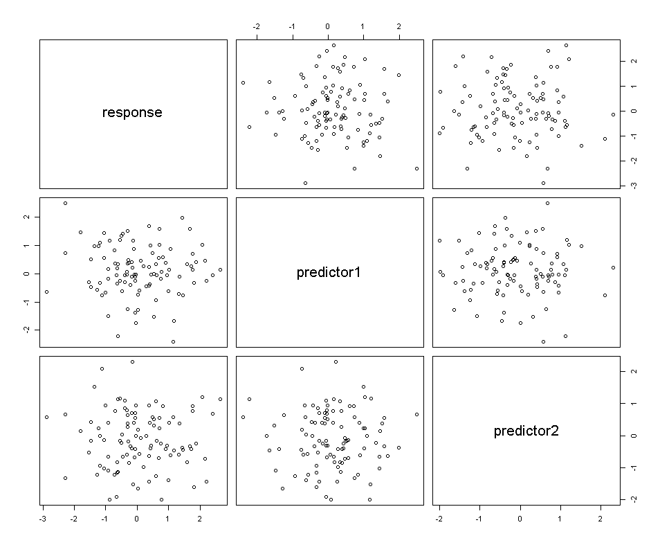

This is a repost of an example that I posted last year but at the time I only had the PDF document (written in Image may be NSFW.
Clik here to view.).  I’m reposting it directly into WordPress and I’m including the graphs.

From time-to-time a researcher needs to develop a script or an application to collect and analyze data. They may also need to test their application under a variety of scenarios prior to data collection. However, because the data has not been collected yet it is necessary to create test data. Creating continuous data is relatively simple and is fairly straight forward using the Cholesky (pronounced kol-eh-ski) decomposition. This approach takes an original X variable (or matrix) and uses the Cholesky transformation to create a new, correlated, Y variable. To make things simple and straight forward this example will generate data from the a random normal distribution N(0,1).

The reason this approach is so useful is that that correlation structure can be specifically defined. The scripts can be used to create many different variables with different correlation structures. The method to transform the data into correlated variables is seen below using the correlation matrix R.

Image may be NSFW.
 Clik here to view.

Once the correlation matrix is set the researcher takes the Cholesky decomposition of the correlation matrix. Multiplying the Cholesky decomposition of the correlation matrix by the data matrix the resulting matrix is a transformed dataset with the specified correlation.

Image may be NSFW.
Clik here to view.
The R code from below will generate a correlation matrix of:

Image may be NSFW.
 Clik here to view.

Image may be NSFW.
 Clik here to view.
R < - matrix(cbind(1,.80,.2,  .80,1,.7,  .2,.7,1),nrow=3)
U <- t(chol(R))
nvars <- dim(U)[1]
numobs <- 100000
set.seed(1)
random.normal <- matrix(rnorm(nvars*numobs,0,1), nrow=nvars, ncol=numobs);
X <- U %*% random.normal
newX <- t(X)
raw <- as.data.frame(newX)
orig.raw <- as.data.frame(t(random.normal))
names(raw) <- c("response","predictor1","predictor2")
cor(raw)
plot(head(raw, 100))
plot(head(orig.raw,100))






To leave a comment for the author, please follow the link and comment on his blog:  Statistical Research » R.

R-bloggers.com offers daily e-mail updates about R news and tutorials on topics such as: visualization (ggplot2, Boxplots, maps, animation), programming (RStudio, Sweave, LaTeX, SQL, Eclipse, git, hadoop, Web Scraping) statistics (regression, PCA, time series,ecdf, trading) and more...